Blog

Market research is an essential activity for every business and helps you to identify and analyse market demand, market size, market trends and the strength of your competition.  It also enables you to assess the viability of a potential product or service before taking it to market. It is a field that recognises the importance of utilising data to make evidence based decisions and many statistical and analytical methods have become popular in the field of quantitative market research.

In our Market Research terminology blog series, we discuss a number of common terms used in market research analysis and explain what they are used for and how they relate to established statistical techniques. Here we discuss “CHAID”, but take a look at our previous articles on Key Driver Analysis, Maximum Difference Scaling and Customer Segmentation, and look out for new articles on TURF and Brand Mapping, coming soon. If there are other terms that you’d like us to blog on, we’d love to hear from you so please do get in touch.

What is it for?

CHAID (Chi-square Automatic Interaction Detector) analysis is an algorithm used for discovering relationships between a categorical response variable and other categorical predictor variables. It is useful when looking for patterns in datasets with lots of categorical variables and is a convenient way of summarising the data as the relationships can be easily visualised.

In practice, CHAID is often used in direct marketing to understand how different groups of customers might respond to a campaign based on their characteristics. So suppose, for example, that we run a marketing campaign and are interested in understanding what customer characteristics (e.g., gender, socio-economic status, geographic location, etc.) are associated with the response rate achieved. We build a CHAID “tree” showing the effects of different customer characteristics on the likelihood of response.

At the first level (the “trunk”) we have all customers and the overall response rate for the marketing campaign was, say, 24.3%. As we progress down the tree to the first “branch”, we identify the factor that has the greatest impact on the likelihood of response, and our overall population is broken down into groups (“leaves”) based upon their differing values of this characteristic – Urban/Rural. We might find that rural customers have a response rate of only 18.6%, whereas urban customers have a response rate of 28.5%. We check to see if this difference is statistically significant and, if it is, we retain these as new leaves. At the next branch, for each of the new groups (Urban/Rural), we then consider whether they can be further split into subgroups so that there is a significant difference in the dependent variable (the response rate). Urban homeowners may have a much higher response rate (36.1%) compared with urban non-homeowners (22.7%), and rural full-time workers might have a higher response rate (24.0%) than rural part-time workers (17.8%) or the rural retired/unemployed (5.3%), for example. At each step every predictor variable is considered to see if splitting the sample based on this factor leads to a statistically significant relationship with the response variable. Where there might be more than two groupings for a predictor, merging of the categories is also considered to find the best discrimination. If a statistically significant difference is observed then the most significant factor is used to make a split, which becomes the next branch in the tree.

The process repeats to find the predictor variable on each leaf that is most significantly related to the response, branch by branch, until no further factors are found to have a statistically significant effect on the response (e.g., likelihood of responding to the marketing campaign). The results can be visualised with a so-called tree diagram – see below, for example. In this case, we can see that urban homeowners (36.1%) have the highest response rates, followed by rural full-time workers (24.0%) and that these are therefore the best groups of customers to target. On the other hand, the lowest response rates were observed for the rural, retired/unemployed, aged over 65 years (1.4%).

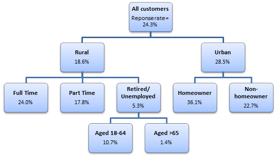
An example of a CHAID tree diagram showing the return rates for a direct marketing campaign for different subsets of customers.

What statistical techniques are used?

As indicated in the name, CHAID uses Person’s Chi-square tests of independence, which test for an association between two categorical variables. A statistically significant result indicates that the two variables are not independent, i.e., there is a relationship between them. (See our recent blog post “Depression in Men ‘Regularly Ignored’…” for an example looking at the relationship between perceived mental health disorders and gender.)

Chi-square tests are applied at each of the stages in building the CHAID tree, as described above, to ensure that each branch is associated with a statistically significant predictor of the response variable (e.g., response rate). Bonferroni corrections, or similar adjustments, are used to account for the multiple testing that takes place. When testing with a 5% significance level (i.e., considering a p-value of less than 0.05 to be statistically significant) we have a one in 20 chance of finding a false-positive result; concluding that there is a difference when in fact none exists (see this light-hearted cartoon for further discussion of multiple testing). The more tests that we do, the greater the chance we will find one of these false-positive results (inflating the so-called Type I error), so adjustments to the p-values are used to counter this, so that stronger evidence is required to indicate a significant result.

CHAID can also be extended to apply to the case where we have a continuous response variable, for example, sales recorded in £’s. However, in this case F-tests rather than Chi-square tests are used. Continuous predictor variables can also be incorporated by determining cut-offs to create ordinal groups of variables, based, for example, on particular percentiles of the variable. So, we might band incomes into four groups, based on its quartiles, such as ≤ £15,000; > £15,000 & ≤ £20,000; > £20,000 & ≤ £33,000; and > £33,000.

Generally a large sample size is needed to perform a CHAID analysis. At each branch, as we split the total population, we reduce the number of observations available and with a small total sample size the individual groups can quickly become too small for reliable analysis.

Alternative methods

When we are interested in identifying groups of customers for targeted marketing where we do not have a response variable on which to base the splits in our sample, we can use other market segmentation techniques such as cluster analysis (see our recent blog on Customer segmentation for further information).

CHAID is sometimes used as an exploratory method for predictive modelling. However, a more formal multiple logistic or multinomial regression model could be applied instead. These regression models are specifically designed for analysing binary (e.g., yes/no) or categorical response variables and can accommodate continuous and/or categorical predictor variables. Interaction terms could be included in the model to investigate the associations between predictors that are tested for in the CHAID algorithm, whilst allowing a wider range of possible model specifications which may well fit the data better. Another advantage of this modelling approach is that we are able to analyse the data all-in-one rather than splitting the data into subgroups and performing multiple tests. In particular, where a continuous response variable is of interest or there are a number of continuous predictors to consider, we would recommend performing a multiple regression analysis instead. See our recent blog post on Analysing Categorical Data Using Logistic Regression Models for further details of these more formal modelling approaches.