Regression to the Mean: as relevant today as it was in the 1900s
The 16th of February marked the anniversary of the birth of Sir Francis Galton, one of the most exceptional statisticians of his time (1822-1911). Whilst Galton may not have the same recognition and fame as some of his fellow scientists (Charles Darwin was his cousin), his scientific achievements were substantial and his influence on statistics is still felt strongly today. Galton introduced many important statistical concepts that are now standard in many statistical analyses; including correlation, standard deviation and percentiles to name a few.
Galton devoted much of his life to the study of variation in human populations and it was during his studies about heredity (the passing of traits from parents to their offspring) that he introduced the concept of regression. However, he did not use this term as statisticians do now (when referring to the fitting of linear relationships); instead he was referring to a very specific statistical phenomenon known as regression to the mean.
Investigating the relationship between the heights of parents and their children, Galton plotted the heights of 930 children who had reached adulthood against the mean height of their parents. To account for differences due to gender he increased female heights by a factor of 1.08.
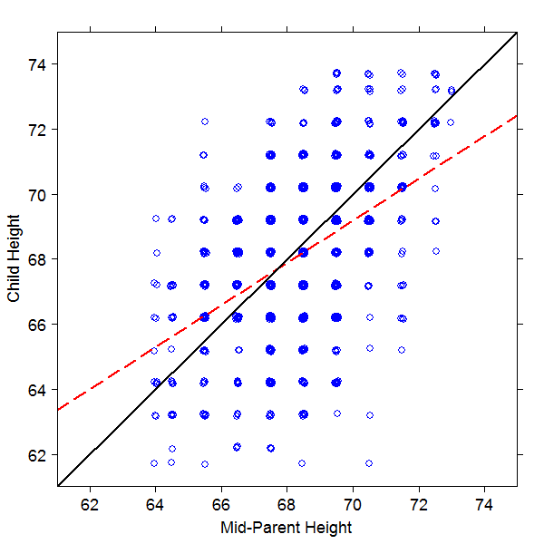
A reproduction of Galton’s plot of Child Height versus Mid-Parent Height.
The above figure is a replication of this plot, where the blue circles represent the height of each child plotted against the mean height of their two parents (which Galton described as the ‘mid-parent height’). Galton grouped the results by intervals of 1 inch, which means that many points are plotted on top of one another. Using Stephen Senn’s approach in his Significance article about Galton, each point has been moved a very small amount in both directions to separate the overlapping points from one another so that it’s easier to visualise where there are many observations plotted at the same point.
When Galton examined this plot he discovered a surprising result. If a child’s height was on average the same as their parents, he would expect the data to follow the black line in the figure above. However, plotting the line of best fit through the data (red dashed line), he found that the data did not follow this black line and that the slope of the least squares fit was in fact less steep. He observed:
“It appeared from these experiments that the offspring did not tend to resemble their parents in size, but always to be more mediocre than they – to be smaller than the parents, if the parents were large; to be larger than the parents, if the parents were small.”
This statistical phenomenon is known as regression to the mean and occurs when repeated measurements are made. It means that, in general, relatively high (or low) observations are likely to be followed by less extreme ones nearer the subject’s true mean. Hence Galton’s use of regression: ‘regress’ means to go back or revert to an earlier or more primitive state.
Regression to the mean remains an important statistical phenomenon that is often neglected and can result in misleading conclusions. For example, official statistics released on the impact of speed cameras suggested that they saved on average 100 lives a year. This result was based on the fall in fatal accidents that had occurred since the cameras had been installed. However, speed cameras are often installed after there have been an unusually high number of accidents and so you would generally expect these to return back to normal levels afterwards anyway. Further analysis that took regression to the mean into account found that 50% of the decline in accidents would have occurred whether or not a speed camera had been installed. This highlights that, although speed cameras may still reduce the number of fatal road accidents, estimating the size of their effect must be done with care.
Regression to the mean is perhaps most easily understood by taking the following example. Suppose you take ten people and give each of them 10 coins. You ask each person to flip each of their coins and to count the number of heads they get. You then take the person who gets the most heads, ask them to wear a silly hat and then get them to flip their coins again. The second time they’ll most likely get fewer heads than before but, of course, it’s nothing to do with the hat you’ve asked them to wear! Regression to the mean occurs here because you’re comparing the number of heads the selected person gets not simply with what they got before, but with the most heads that any of the 10 observed. You’ve deliberately picked an extreme number of heads and it’s almost inevitable that when trying again, they’ll get fewer heads the second time.
The trick to dealing with regression to the mean is to make sure that you always compare like with like. If you only take action when something unusual happens then you need to take account of that fact when assessing the impact of that action. The key is to determine a baseline measurement that you can compare before or after treatment so that you’re comparing measurements not against past extremes, but against what you might otherwise expect. In many cases this can be done by using control groups or by modelling past data to gain a better understanding of the baseline effect against which you can compare.